The acceleration may be calculated by using two consecutive intervals. Let t1 be the first time interval of the two consecutive intervals and t2 be the second time interval of the two consecutive time intervals. Let the constant distance interval be represented by s. If the acceleration, a, is constant, then the equations of a uniformly accelerated motion apply. For the first interval the following equation applies:
s = v1i t1 + at1 2 ⁄ 2 . . . . . .(1)
where v1i is the initial velocity of the first interval. And for the second interval the following equation applies:
s = v2i t2 + at2 2 ⁄ 2 . . . . . .(2)
where v2i is the initial velocity of the second interval. The final velocity, v1f, of the first interval is the same as the initial velocity, v2i, of the second interval. Therefore,
v2i = v1f = v1i + at1 . . . . . .(3)
Substituting equation (3) into equation (2) we obtain
s = v1it1t2 + a ( t1t2 + t1 2 ⁄ 2 ) . . . . . ( 4 )
The time intervals, t1 , t2 and the constant distance interval, s, will be measured. Thus, we will have only two unknowns, v1i and a, in equations (1) and (4). That means we can solve for the acceleration a simultaneously in terms of t1 , t2 and s to obtain
a = 2s ( t1 - t2 ) ⁄ [ t1 t2 ( t1 + t2 ) ] . . . . . ( 5 )
That is, if two consecutive time intervals and the constant distance interval are measured, the acceleration can be calculated.
Once the acceleration has been calculated, the initial velocity, v1i , of the first interval can be obtained from equation (1) as:
v1i = s ⁄ t1 - at1 ⁄ 2 . . . . . ( 6 )
Similarly the initial velocity of the second time interval, v2i , (or the final velocity of the first interval, v1f ) may be obtained from:
v2i = v1f = v1i + at1 ⁄ 2 . . . . . (7)
And substituting for v1i from equation (6) into equation (7) we get
v2i = v1f = s ⁄ t1 + at1 ⁄ 2 . . . . . ( 8 )
The final velocity of the second interval, v2f , may be calculated from
v2f = v2i + at2 . . . . . ( 9 )
And substituting for v2i from equation (8) into equation (9) we obtain
v2f = s ⁄ t1 + a ( t1 + 2t2 ) ⁄ 2 . . . . . ( 10 )
ME = KE + PE . . . . . ( 11 )
The principle of conservation of mechanical energy may be mathematically written as
MEf = MEi
or
KEf + PEf = KEi + PEi . . . . . ( 12 )
Where MEi , KEi and PEi are the initial mechanical, kinetic and potential energies respectively and MEf , KEf and PEi are the final mechanical, kinetic and potential energies respectively.
The kinetic energy, KE, of an object of mass m and speed v is given by
KE = mv 2 ⁄ 2 . . . . . ( 13 )
And if the conservative force acting on the system is gravitational force, the potential energy, PEg , of an object of mass m and y-coordinate (vertical coordinate) y with respect to a certain reference point (choice of reference point is arbitrary as far as the same reference point is used consistently) is given by
PEg = m|g|y . . . . . ( 14 )
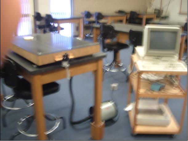
In this experiment, the system will involve an object of mass m1 sliding on an air table attached to a hanging object of mass m2 via a string. The force of friction acting on the sliding object will be reduced to a minimum by means of a blower and can be neglected. Thus, the only force with non-zero contribution to the work done acing on the system is the force of gravity acting on the hanging object (the normal force exerted by the surface of the table on the sliding object has no contribution to the work done because it is perpendicular to its trajectory). Therefore, since gravity is a conservative force, the mechanical energy of the system is conserved.
Both objects will be moving with the same speed, . Thus, the kinetic energy of the system is given by
KE = ( m1 + m2 ) v 2 ⁄ 2 . .. . . ( 15 )
If the y-coordinate of the sliding object is y1 and the y-coordinate of the hanging object is y2 , then the potential energy of the system is given by
PE = m1 |g|y1 + m2 |g|y2 . . . . . ( 16 )
Now the conservation of mechanical energy for this system may be obtained by substituting equations (15) and (16) into equation (12).
( m1 + m2 ) vf 2 ⁄ 2 + m1 |g|y1f + m2 |g|y2f = ( m1 + m2 ) vi 2 ⁄ 2 + m1 |g|y1i + m2 |g|y2i . . . . . ( 17 )
Since m2 is sliding in a horizontal surface, its y-coordinate will not change; that is y1f = y1i and equation ( 17 ) reduces to
( m1 + m2 ) vf 2 ⁄ 2 + m2 |g|y2f = ( m1 + m2 ) vi 2 ⁄ 2 + m2 |g|y2i . . . . . ( 18 )
or
{ ( m1 + m2 ) vf 2 ⁄ 2 + m2 |g|y2f } ⁄ { ( m1 + m2 ) vi 2 ⁄ 2 + m2 |g|y2i } = 1 . . . . . ( 19 )
hanger mass ( m2 ) = kg = 0.005 kg
first time interval ( t1 ) = s
second time interval ( t2 ) = s
Record t1 on the first row of column 2 and t2 on the first row of column 3 of the Table .
a = 2s ( t1 - t2 ) ⁄ [ t1 t2 ( t1 + t2 ) ]
Using the time intervals, t1 and t2 obtained in procedure (9.) and the distance of one interval ( s ) obtained from procedure (2.), calculate the acceleration of the system.
acceleration ( a ) = 2s ( t1 - t2 ) ⁄ [ t1 t2 ( t1 + t2 ) ] = m ⁄ s 2
Record this on the first row of column 4 of the table.
Table 1
update table